From Trade Log to Verdict: The Statistics of a Significant Edge

A standalone tutorial on the statistical techniques in crucible: how each one contributes to declaring a trade log statistically significant, worked end to end on an example system, with references to the source literature.

📄 Download this tutorial as a PDF · 🎧 Prefer to listen? The podcast companion →

Running the code. Everything on this page runs on pip install crucible. The two end-to-end scripts (§12, §13) live in the repo under examples/ and use reproducible synthetic data, so python examples/donchian_gauntlet.py reproduces the exact numbers you see here, with no network and no data of your own.

---

0. What "statistically significant trade log" actually means

A backtester hands you a rising equity curve and a headline number: "profit factor 1.37, 214 trades." The number is real in the sense that it happened on the data. The question this tutorial is about is different:

Given how few trades I have, and how many variants I tried before landing on this one, could a curve this good have come from no edge at all?

Answering that turns a point estimate into a verdict. Two distinct failure modes have to be ruled out (the framing is Aronson's):

1. Luck mistaken for skill: a small sample, or a large search, threw up a good number by chance. (Statistical validity.)
2. A real pattern that doesn't travel: genuine in-sample, gone out-of-sample or on another market. (Robustness / generalization.)

crucible answers these at the trade-log level, before any capital, position sizing, or equity curve enters the picture. Everything here is capital-free. The concepts come first (§1–§11). Then §12 works the whole pipeline end to end on a Donchian breakout, so you can see exactly how to read every number and verdict.

If you're coming from a backtester

Every number your backtester hands you describes. Nothing here disputes them. A profit factor of 1.37 on 214 trades is an arithmetic fact about what happened. The question is whether those numbers can defend themselves: whether they would still be there once the luck, the search, and the market's own drift are taken away. That arc, describe → defend, is the whole tutorial, and it maps onto the pipeline below exactly: the first stage describes the edge, and every stage after it defends the description.

Most of what you already have maps onto something here:

what you have	what crucible asks of it
the equity curve	the R-multiple trade log underneath it (§1)
"profit factor 1.37"	the same 1.37 with a CI around it. STRONG gates its lower bound against 1.25, not the point estimate (§2–§3, §11)
the optimizer's trial count	n_variants, which you declare, and nothing counts it for you (§5b)
the walk-forward report	DURABLE: the WFE and the fold dispersion (§9)
Monte Carlo on the equity curve	the sign-permutation p, a different question entirely (§5a)
position sizing, drawdown, ruin	out of scope, the SURVIVE handoff (§11)
"it passed"	HELD / FRAGILE / FAIL (§4)

The Monte Carlo row is the one to slow down on, because it's the one you think you've already done. Your backtester's Monte Carlo takes your trades and reshuffles their order, into thousands of alternate sequences, a spread of drawdowns and final equities. Notice what never changes: every one of those curves is built from your wins and your losses. Your winners stay winners. The edge is assumed, and the question is how rough the ride around it could get. That's a real and useful question. It's just a question about sequencing risk, and it cannot tell you the edge exists, because it began by granting it.

The sign-permutation test grants nothing. It keeps each trade's magnitude and flips its sign at random. A coin decides whether each trade won or lost. That builds the world where you had no directional skill whatsoever but the same trade sizes and the same volatility. Rebuild that world ten thousand times, and count how often it matches or beats what you actually got. That fraction is p. When §12's Donchian breakout comes back at p = 0.0008, it means: in a world with no edge at all, a result this good turned up 8 times in 10,000.

So the two are near-opposites in what they assume. Monte Carlo assumes the edge and measures the ride. Permutation assumes no edge and asks whether your results could have happened anyway. This is why a strategy can sail through your Monte Carlo and still fail REAL. The MC never tested the thing REAL tests.

The names collide, unhelpfully. §5a's technique is Monte Carlo, and Masters calls it the Monte Carlo Permutation Method. "Monte Carlo" is just the machinery: randomize, repeat, count. What separates the two is what you randomize and what you hold fixed. Your backtester randomizes the order and holds the outcomes fixed. The permutation test randomizes the outcomes and holds the magnitudes fixed. Same machinery, opposite question.

§12 is this table run end to end, a Donchian breakout that hands you 162 trades and a profit factor of 1.90, and then has to defend them.

Everything below is organized as a pipeline: describe the edge → quantify sampling noise → rule out data-mining luck → rule out drift → confirm out-of-sample → account for correlation. Each section names the technique, the code that implements it, the statistical logic, and where to read the primary source.

---

1. The substrate: a risk-normalized trade log (R-multiples)

Your trades are denominated in dollars. Everything downstream needs them in units of risk. This is that conversion.

Code: edge/trade_log.py, edge/simulator.py

Every technique downstream operates on one object: a TradeLog whose required column r is the per-trade return in R-multiples, profit measured in units of the risk taken at entry, the entry-to-stop distance (1R = entry − stop, which the barrier simulator sizes as sl × ATR). R-normalization is what lets returns from different instruments and volatility regimes pool into one sample that the statistics can treat as draws from a single distribution.

The unit that defines 1R is just the strategy's own stop, and crucible is agnostic to how it's set: a volatility statistic (ATR, the simulator's default), a structural level (a swing low or reversal-candle wick), or a fixed distance. All are valid risk units. The volatility-scaled framing holds specifically when that unit is a volatility measure like ATR. A structural stop is risk-normalized but only implicitly volatility-sensitive (a wider signal bar gives a wider stop).

Subtract costs before you test. The r column should be net of transaction costs, commission and slippage, expressed in R. A fixed haircut (say −0.1R per trade for a liquid instrument, more for thin ones) is the floor. Without it a +0.15R expectancy might be literally just the spread, and every p-value downstream is defending a phantom edge. The bias is worst exactly where it looks best: the same dollar of slippage is a larger fraction of a tight-stop (small-R) trade, so cost-per-R is highest on the highest-expectancy setups. crucible is capital-free but not cost-free. Net the haircut into r before the gauntlet ever sees the log. (Sizing-dependent frictions, financing and market impact at size, belong to the capital layer, §10.)

The netting is a few lines on what a backtester already hands you per fill, the gross R, and the entry and stop that defined 1R. A round turn costs a fixed dollar amount, so in R it is that dollar cost over the dollars you had at risk:

cost_usd = commission + 2 * slippage_ticks * tick_value   # round-turn $, e.g. $5 + 2·1·$10 = $25
risk_usd = abs(entry - stop) * point_value                # the dollars 1R actually risked
r_net    = r_gross - cost_usd / risk_usd                  # cost in R = $cost / $risk

Dividing by risk_usd is the whole point. It is what makes the flat-haircut shortcut above a floor, not the truth. Take gold ($100/point, $10/tick, so the same $25 round turn on every trade):

• a wide 15-point stop risks $1,500 → cost $25 / $1,500 = 0.017R → a +0.15R edge nets +0.133R (−11%)
• a tight 3-point stop risks $300 → cost $25 / $300 = 0.083R → the same +0.15R edge nets +0.067R (−56%)

Same instrument, same $25, and the tighter-stop book, the one that looked better gross, loses more than half its edge. A flat −0.1R can't see that. Charging per dollar-of-risk can, which is what a full futures cost layer does per trade (pricing each fill from its own risk and the contract's tick/point value, with an extra tick for thin markets), stamping the result on the verdict: "net of 0.06R/trade."

Because crucible only ever sees the r you hand it, it can't tell a net log from a gross one, so it never assumes. A gauntlet report whose log carries no cost attestation is stamped costs not attested. A producer that has already netted says so, and crucible repeats the claim. Netting stays yours to do. The verdict just refuses to hide whether you did.

The TradeLog is deliberately agnostic about how the trades were produced. A hand-coded moving-average rule, a set of discretionary fills exported from a broker or a RealTest run, and an ML take/skip filter all reduce to the same schema, a column of R-multiples (plus optional MFE/MAE, holding period, entry/exit dates). The honesty layer never sees the strategy. It sees only the returns, which is exactly why one set of tests serves rule-based and model-based books alike.

When you do generate the log from an entry rule, the barrier simulator that manufactures it is deliberately look-ahead-free: barriers are sized off the signal bar (the bar the rule fires on, known at entry), and exits are scanned forward from the entry bar (simulator.py:64, :75). This matters because every p-value later assumes each r was knowable only at the moment of the trade. A single peek into the future contaminates the whole null distribution.

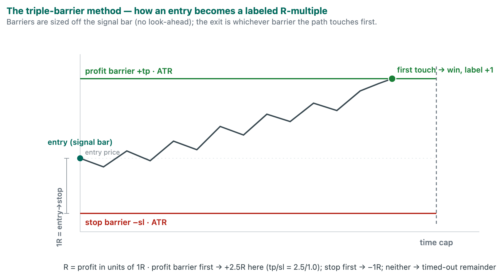Each entry is scored by whichever barrier fires first: a profit target (+tp·ATR), a stop (−sl·ATR), or a time cap. The same construction labels trades for the ML track (§7).

Sources. The R-multiple as the unit of trade evaluation: Van Tharp, Definitive Guide to Position Sizing (2008), Ch. 2 "Risk (R) and R-Multiples" (p. 11). Popularized in Trade Your Way to Financial Freedom (2nd ed. 2007). Risk-normalized, volatility-scaled return accounting: the ATR-based risk unit (1R = sl × ATR) is the trade-log echo of Carver, Systematic Trading, Ch. 9 "Volatility Targeting", the same volatility unit, applied to measuring each trade rather than sizing it (position sizing itself is the SURVIVE handoff, §11. Its sources are in §10). The leakage-free barrier construction is the same geometry ML uses to label forward outcomes (López de Prado, Advances in Financial Machine Learning, §3.4 "The Triple-Barrier Method", cross-referenced in §7), but here it turns any entry rule into trades, ML or not.

---

2. Describing the edge: capital-free metrics

The numbers your backtester already prints, defined precisely enough to be tested.

Code: edge/metrics.py

Before any significance test, you summarize the sample. These are point estimates. They describe, they do not yet defend.

Metric	Definition (code)	Reads on
Expectancy	wr·avg_win − lr·avg_loss (in R), metrics.py:28	mean profit per trade
Profit factor	gross win / gross loss, :41	reward-to-risk of the whole book
Payoff ratio (a.k.a. RR / risk-reward)	avg win / avg loss, :51	terminal reward-to-risk geometry
Win rate	fraction of r > 0, :23	how often you're right, read with payoff, never alone (35% is excellent at RR 3)
SQN	mean/std · √min(n,100), :60	signal-to-noise, the risk-adjusted quality score
MFE (max favorable excursion)	per trade: furthest it ran for you while open, in R. A trade-log column the simulator records (simulator.py)	the unrealized profit that was on the table
MAE (max adverse excursion)	per trade: furthest it ran against you while open, in R (≤ 0). Simulator column	the worst heat taken to hold it
Excursion / E-ratio	mean MFE / mean|MAE|, :76,:85	is there directional edge before the exit rule?
Time asymmetry	avg bars in wins / avg bars in losses, :91	"let winners run, cut losers"
Exit efficiency	captured / available MFE, :102	how much of the move the exit banked

The one to single out is SQN (System Quality Number, Van Tharp): mean(R) / std(R) × √n. It is a Sharpe-like t-statistic on the per-trade returns, the same quantity a significance test formalizes. A high mean means nothing if the standard deviation is huge or n is tiny. SQN is the first hint of whether the sample can support a claim at all.

What's deliberately absent: drawdown. You won't find max drawdown, CAGR, or risk-of-ruin in this table, and that's on purpose. Drawdown is a function of position sizing and capital, not raw edge: two books with the identical r column can have wildly different drawdowns depending only on how big and how concurrently you size them (correlated positions open at once cluster their losses). So drawdown/ruin belong to the SURVIVE (capital) layer, the block-bootstrap portfolio Monte Carlo of §10 and beyond, not to this raw-edge layer. crucible measures the edge. What it costs you to hold it is a separate question.

Sources. - Expectancy, profit factor, payoff, drawdown and the rest of the classic evaluation battery: Pardo, The Evaluation and Optimization of Trading Strategies, 2nd ed. (2008), the "Evaluation of Trading Strategies" chapter. This is the canonical list edge_report reproduces. - SQN: Van Tharp, Definitive Guide to Position Sizing (2008), Ch. 3 "Evaluating the Quality of Your Trading System" (p. 23), and, precisely on the small-sample problem the √min(n,100) cap addresses, "One Problem with System Quality Number and How to Overcome It" (p. 32) and "Statistical Assumptions in Using This Material" (p. 33). Popularized in Trade Your Way to Financial Freedom (2007). crucible's sqn() (metrics.py:60) uses Van Tharp's √min(n,100) cap. (A √100-always variant would inflate a 30-trade SQN by √(100/30) ≈ 1.8×, crediting it with confidence it hasn't earned. The actual trade count is the honest scale.) - Excursion (MFE/MAE) analysis: Sweeney, Campaign Trading. Curtis Faith, Way of the Turtle (the E-ratio), cited in the metrics.py module docstring. - The risk-adjusted framing (why std matters as much as mean): Carver, Advanced Futures Trading Strategies (2021), the chapters on the Sharpe ratio and evaluating returns. Carver stresses that a Sharpe/SQN is itself an estimate with a wide error bar, which is exactly what §3 addresses.

---

3. Quantifying sampling noise: the bootstrap confidence interval

You have one number from a couple of hundred trades. This asks how much of it is the sample.

Code: edge/stats.py. bootstrap_ci, p_value_positive, and bootstrap_metric_cis (the whole metric set in one resample pass).

A point estimate of expectancy on 60–200 trades badly understates how much it could have wobbled. The bootstrap turns the single number into a distribution:

for i in 1..10000:           # stats.py:65  _resample
    draw = sample r WITH REPLACEMENT, size n
    record metric(draw)
CI = [2.5th percentile, 97.5th percentile]     # stats.py:87

Resampling the trade log with replacement simulates "other histories you could plausibly have drawn from the same edge." The 2.5–97.5 percentile band is the 95% confidence interval. p_value_positive reports the fraction of resamples where the metric stayed positive.

Why it is the honest read: it makes no normality assumption (trade returns are skewed and fat-tailed), and it works for any metric (expectancy, profit factor, SQN), not just the mean. On small samples the band is wide, and that width is the message.

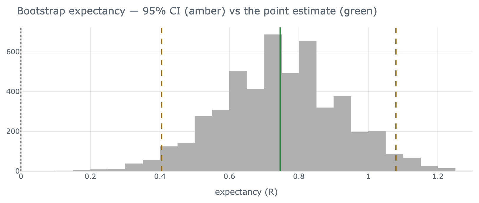The bootstrap made visible. This is the report's "Bootstrap expectancy" panel (§11) for the worked example's out-of-sample log. Each grey bar is one resample's expectancy. The dashed amber lines are the 2.5/97.5-percentile 95% CI, the green line the point estimate, the dotted line zero. Here the whole band sits right of zero. The edge holds across resamples (the HELD read of §4). When the amber lower line crosses left of zero, that's FRAGILE. This panel is the i.i.d. bootstrap (it resamples individual trades). For a pooled multi-asset book the honest, wider band comes from block_bootstrap_ci (below) and is not drawn here.

crucible's gauntlet gates on this: its STRONG gate requires the CI lower bound, not the point estimate, to clear each threshold (gate_strong, §11). This directly fixes the "PF 1.37 on 60 trades treated as a clean pass" failure: a positive point estimate whose CI lower bound is negative does not clear the gate.

Sources. - Aronson, Evidence-Based Technical Analysis (EBTA, 2006), Ch. 4 "Statistical Analysis" (p. 165) and Ch. 5 "Hypothesis Tests and Confidence Intervals" (p. 217), sampling distributions, the bootstrap, and confidence intervals for trading statistics. This is the direct antecedent of bootstrap_ci. - AFML Ch. 14 "Backtest Statistics", the family of statistics a backtest should report as distributions, not points. - Carver, Systematic Trading, Appendix C "Portfolio Optimisation → More details on bootstrapping", bootstrap resampling applied to strategy/portfolio estimates.

When the observations aren't independent: the block bootstrap

The i.i.d. bootstrap above (and the sign-permutation of §5) treats trades as exchangeable: i.i.d. means independent (one trade's outcome carries no information about the others) and identically distributed (all drawn from one fixed distribution), so their order doesn't matter and you can resample them one at a time. That's fine for a single instrument, but it breaks for a pooled multi-asset book: one macro shock in Oct-2008 fires correlated longs across equities, metals, and FX at once, so those trades are not independent draws. Resampling them independently overstates the edge's significance, too-tight CIs, too-small p.

The fix is to resample contiguous blocks of calendar time instead of individual trades, so the clustering survives in the null. Feed block_bootstrap_pvalue / block_bootstrap_ci (edge/stats.py) an ordered period-return series (e.g. monthly summed R on a gap-free grid), and it zero-centers to impose the null (mean = 0) and resamples blocks (circular, or the Politis–Romano stationary bootstrap for random block lengths):

from crucible.edge import block_bootstrap_pvalue
p = block_bootstrap_pvalue(monthly_R, block=6)   # ~1 ≈ i.i.d.; larger blocks absorb autocorrelation

block≈1 reproduces the i.i.d. result. Longer blocks widen the null exactly when the series is positively autocorrelated, the honest p for a clustered book. Useful diagnostic: if the p barely moves as the block grows, the clustering is hurting your drawdown, not the significance of your mean, two different statistics.

The report draws this comparison directly: pass a period series to the tearsheet (edge_panels(trades, period_returns=monthly_r(trades)), or the same argument on gauntlet_report) and it appends a block-bootstrap panel that shows the wider, correlation-preserving CI against the optimistic i.i.d. one on the period-mean axis, the picture of "the i.i.d. band is too tight" rather than just the assertion.

Source. Politis & Romano (1994), "The Stationary Bootstrap," JASA 89(428): 1303–1313, the block/stationary bootstrap for dependent data (Bootstrapping (statistics)).

---

4. The verdict: folding point + CI + p-value into a label

Your backtester said "profitable." This turns that into HELD, FRAGILE or FAIL, and means it.

Code: edge/stats.py. reality_check, Verdict (stats.py:44)

reality_check is the call the README calls "the whole point of the package." It collapses the three numbers into a decision:

HELD     point > 0  AND  CI lower bound > 0     # the edge clears zero across resamples
FRAGILE  point > 0  BUT  CI straddles zero       # positive, but indistinguishable from noise
FAIL     otherwise

FRAGILE is the state a backtester never shows you: a positive expectancy whose confidence interval includes zero. The equity curve looked like an edge. The statistics say don't size it up. This is significance testing expressed as an operating instruction rather than a p-value to be argued over.

Sources. The philosophy (a rule earns belief only when the evidence clears a pre-set statistical bar, not when it merely looks good) is the thesis of EBTA Ch. 3 "The Scientific Method and Technical Analysis" (p. 103) and Ch. 5 (p. 217). The "hard gate, no discretionary override" posture is the gauntlet's own (§11): a failing hard check can't be waived by a reviewer who likes the strategy.

---

5. Ruling out data-mining luck: permutation tests

You tried forty things and kept the best one. This section prices that.

This is the heart of the significance story and the reason Aronson & Masters matter.

First, a lens: what does the test hold fixed?

§0 took your backtester's Monte Carlo apart with two questions: what does it randomize, and what does it hold fixed? That lens isn't special to Monte Carlo. It is how every test in this tutorial works, and it's the fastest way to know what one can and cannot tell you. Each test builds a world and drops your results into it. What it holds fixed is what it grants you for free. What it randomizes is the thing whose contribution it is actually measuring. Sorted that way, the whole toolkit is three families.

1. Resample your own trades. These grant your results and ask how much of the number is noise.

test	holds fixed	randomizes	answers
bootstrap_ci (§3)	your trades, treated as the population	which trades you drew	how much of the number is the sample
block_bootstrap_ci (§3)	contiguous blocks of calendar time	which blocks you drew	the same, with autocorrelation left intact
your backtester's Monte Carlo	the outcomes themselves	their order	how rough the ride could get

2. Build a world where you had no skill. These grant nothing. This is where "is the edge real?" actually gets answered.

test	holds fixed	randomizes	answers
sign_permutation_pvalue (§5a)	each trade's magnitude	its sign	is there directional skill at all
random_entry_null (§6)	the prices, the barriers, the trade count, the holding period	when you entered	timing skill, or just exposure
detrended_timing_null (§6)	your directions and holding periods	timing, on drift-removed returns	timing skill once the market's own drift is gone
block_bootstrap_pvalue (§3)	the block structure	which blocks, zero-centered to impose a no-edge null	the same, for a serially dependent book

3. Correct for how hard you looked. These grant that you found something, and ask whether the finding survives the size of the search that found it.

test	holds fixed	randomizes	answers
whites_reality_check (§5c)	the whole variant pool	signs across every variant, keeping the max	did the size of my search manufacture this winner
Hansen's SPA (§5d)	the same pool, studentized, clear losers dropped	the same	the same question, without one wild variant setting the bar
cross-market RC (§5e)	the markets, used as the variant pool	the same, best market vs best-under-null	does it travel, or is one market carrying the book
PBO (§5, below)	the config pool	which period blocks are IS vs OOS (it enumerates every symmetric split rather than sampling)	did the act of choosing the winner overfit

(§5b's Šidák correction is the odd one out. It randomizes nothing at all. It's the arithmetic shortcut for family three when the only thing you know is the count.)

Now read the first table against the other two. Your backtester's Monte Carlo sits in family one, and it is the only test here that holds the outcomes fixed, which is exactly why it can measure the ride but never the edge. It grants the thing in question. Families two and three are what crucible adds, and no amount of family-one resampling is a substitute for them: they are different questions, not stronger versions of the same one.

§5a is the family-two test, the blunt question, is there any edge at all? Everything after it (§5b onward) is family three, correcting for how hard you looked.

5a. Sign-permutation test (one strategy)

Code: validation/permutation.py. sign_permutation_pvalue

observed = mean(r)
for k in 1..5000:                              # permutation.py:42
    flip each trade's sign at random (±1)
    record mean(signs · |r|)
p = (# permuted means ≥ observed + 1) / (N + 1)

The null hypothesis is "no directional skill". Under it, each trade's sign is a coin flip while its magnitude is whatever it was. Shuffling signs builds the distribution of outcomes a skill-less system would produce on these same magnitudes. The p-value is how often chance matches or beats you. This is Timothy Masters' Monte Carlo Permutation Method, the public-domain alternative to White's patented Reality Check.

In the gauntlet this is the REAL gate's corrected_pvalue hard check: the sign-permutation p, Šidák-corrected (§5b) for your variant count, must clear α = 0.05. On the report it's the corrected_pvalue row in the REAL block, with the raw sign-permutation p in its detail line. (Hand gate_real every variant's returns instead and it swaps to White's Reality Check, §5c, as reality_check_pvalue.)

5b. Šidák correction (you tried N variants)

Code: permutation.py:47. sidak_correction. corrected = 1 − (1 − p)^N

If you quietly tried 50 parameter sets and reported the best, its raw p-value is a lie of selection. Šidák asks: what's the chance the best of N independent searches looks this good by luck? It is the conservative fallback when you only know the count of variants. crucible's REAL gate applies it in the gauntlet. Pass your n_variants (the total number of configs you searched, discards included).

n_variants counts you, not just a grid. If you came from an optimizer, "trials" means grid points, and the tool counted them for you. Here it means every version you tried and rejected: the filter you added because the drawdown looked ugly, the stop you widened after seeing the stop-outs, the two markets you quietly dropped. Those are searches. They leave no log, which makes them more dangerous than a grid, not less: n_variants is a number you supply (gauntlet.py:89), and nothing in crucible can check it. An honest 40 you had to admit to beats a comfortable 4.

5c. White's Reality Check (you have every variant's returns)

Code: permutation.py:59. whites_reality_check

for each permutation:                          # permutation.py:84
    flip signs for EVERY variant
    record the BEST mean across all variants   # the max-statistic
compare observed best against this "distribution of the best"

Taking the maximum inside each permutation is what corrects for the size of the search: you compare your winner not against zero, but against the best number a pure-noise search of the same size would have thrown up. The docstring's warning is load-bearing. You must pass every variant including the discards, or the correction is toothless.

Sources. - EBTA Ch. 6 "Data-Mining Bias: The Fool's Gold of Objective TA" (p. 255), the definitive treatment of data-mining bias, the Monte Carlo permutation method, and White's Reality Check, applied in the Ch. 8 case study (p. 389) across 6,402 rules. - EBTA Acknowledgments (p. ix) credits Timothy Masters with innovating the Monte Carlo permutation method and placing it in the public domain, the exact method in sign_permutation_pvalue. - Aronson & Masters, Statistically Sound Machine Learning for Algorithmic Trading (SSML, 2013), the applied companion. See the Introduction's "Performance Criteria" and the permutation-test / selection-bias sections (the book is organized by topic around the TSSB tool). - White, H. (2000), "A Reality Check for Data Snooping," Econometrica 68(5), the original max-statistic bootstrap whites_reality_check reimplements. (No dedicated Wikipedia page. The problem it corrects lives at Data dredging.) - Multiple-comparisons / overfitting the search itself: AFML Ch. 11 "The Dangers of Backtesting" and Ch. 12 "Backtesting through Cross-Validation."

5d. Superior Predictive Ability: WRC's more powerful successor

Code: permutation.py. spa_test

White's Reality Check has a well-known weakness: it compares raw means and lets every variant (including obvious losers) into the max-under-the-null, so padding the search with junk actually weakens the test (the null max is inflated by noise the winner must beat). Hansen's Superior Predictive Ability (SPA) test fixes both:

• Studentize: divide each variant's mean by its standard error before the max, so a volatile / low-N variant can't dominate just by being noisy.
• Exclude the clearly-inferior: variants whose studentized mean sits far below zero (< −√(2·ln ln N)) are dropped from the null max (the consistent SPA_c recentering), so junk no longer dilutes the test.

The consequence is one-directional: SPA p ≤ WRC p. SPA is (weakly) more powerful. crucible ships spa_test alongside whites_reality_check, not as a replacement, because the extra power cuts against a distrust-first framework's grain. WRC is the conservative number (it errs toward not rejecting). SPA is the powerful one. Report both: stake a deploy on the conservative WRC verdict, and read SPA as "…and it's even stronger under the more powerful test." Reach for SPA especially when the variant pool is heterogeneous (wildly different sample sizes / variances across markets), where studentization matters most.

Sources. - Hansen, P. R. (2005), "A Test for Superior Predictive Ability," J. Business & Economic Statistics 23(4): 365–380, the SPA test spa_test reimplements. No dedicated Wikipedia page. See Peter Reinhard Hansen (whose bio describes the test) and, for the data-snooping problem it corrects, Data dredging.

5e. Cross-market Reality Check: the GENERAL gate

Code: gauntlet.py. gate_general (which calls whites_reality_check / spa_test)

The tests above correct for one search: the parameter/config variants you tried. But a book that applies one universal rule across many markets is running a second, implicit search: testing 28 markets is 28 shots at a winner. The GENERAL gate asks whether the edge travels, and prices that second search exactly as §5c/§5d price the first.

It's the same max-statistic idea, one axis over: treat each market's per-trade returns as a variant and run the Reality Check (or SPA) across them. The pass bar is that the best market beats the distribution of the best under no skill across every market tested, so one lucky market can't carry the book:

variant_returns = {market: its trade returns}     # one entry per market
p = whites_reality_check(variant_returns)          # best market vs best-under-null over N markets
#   gauntlet.py: gate_general  (spa_test is the studentized, more-powerful alternative)

Two things make it honest, and easy to misread:

• Pass every market, including the failures. Which were development vs. held-out is your record to keep, not crucible's (same rule as §5c). Omitting the losers biases it toward a false pass.
• It scores the single BEST market, not the pool. For a pooled, thin-per-market book (the edge lives in the aggregate, ~30 trades/market) that's a stringent, arguably mismatched bar: you can have a genuinely broad, real pooled edge and still have no single market clear an N-way correction. Read a GENERAL failure as "no single market is an individually-validated standout," not "the edge is fake". The pooled edge is REAL/STRONG's job (§5/§3), and breadth is better read two other ways: the book's effective N (§10) and a plain sign test over the units (how many are individually positive).

Choose the unit deliberately. Per symbol is thin (few trades each → almost nothing passes). Per asset class pools within each class into a powered unit and is usually the honest lens. And because markets are wildly heteroskedastic (hundreds of trades in one, a handful in another), this is exactly where SPA's studentization (§5d) earns its keep. On a real 28-asset book, moving the GENERAL unit symbol → class and the test WRC → SPA walked the p from 0.20 → 0.07 → 0.002.

Sources. White (2000) / Hansen (2005) as in §5c–5d. The "does the edge travel across markets" (cross-sectional generalization) framing is the held-out-asset step of AFML Ch. 11–12.

Did the selection overfit? PBO & deflated Sharpe

Code: validation/pbo.py. pbo_cscv, deflated_sharpe

White's Reality Check asks whether the best variant's edge is noise. Two companion tools ask the complementary question: given that you searched N configs and kept the best-in-sample one, how much did the act of choosing overfit?

• PBO, Probability of Backtest Overfitting (pbo_cscv) via Combinatorially-Symmetric Cross-Validation. Feed a T×N performance matrix (periods × the configs you searched). Over every symmetric IS/OOS split of the period blocks it picks the best-in-sample config and reads its rank out-of-sample. PBO is the fraction of splits where the in-sample winner lands below the OOS median. Read it in bands, ROBUST (≤0.10) / GUARDED / OVERFIT, not to the decimal, and (like White's) pass every config you tried or it reads optimistic.

• Deflated Sharpe Ratio (deflated_sharpe). The winner's Sharpe must clear a bar that rises with the number of trials: SR0 is the expected maximum Sharpe of N noise trials, and the DSR is the probability the winner's true Sharpe beats it, corrected for the return series' own skew and kurtosis (fat left tails widen the error bar). Read ≥ 95% like a passed significance test.

Where the permutation test corrects the p-value for the search, these correct the IS ranking and the Sharpe for it, the same multiple-testing disease, caught two more ways. Capital-free (stdlib NormalDist, no scipy).

Unlike the trade-log tests, these two aren't drawn on the report or wired into the gauntlet. They need the whole search as input (pbo_cscv a T×N periods×configs matrix. deflated_sharpe the winner's Sharpe plus the trial count), which a single TradeLog doesn't carry. Call them yourself with that matrix, same story as the block bootstrap (§3): a standalone check that runs on a different object than the one the report shows.

Sources. PBO / CSCV: Bailey, Borwein, López de Prado & Zhu (2017), "The Probability of Backtest Overfitting," Journal of Computational Finance. AFML Ch. 11–12. Deflated / Probabilistic Sharpe: Bailey & López de Prado (2014), "The Deflated Sharpe Ratio," Journal of Portfolio Management, and (2012) the Probabilistic Sharpe Ratio. AFML Ch. 14 "Backtest Statistics."

---

6. Ruling out drift: the random-entry / detrended benchmark

Did you have timing skill, or just exposure? This answers it without picking a benchmark.

Code: edge/stats.py. random_entry_null, detrended_timing_null

Your system made money in a market that went up. This section is about separating those two facts, because your equity curve cannot.

That is an uncomfortable sentence, so be precise about the claim: nobody is saying the money wasn't made. The question is who made it. Take your rule away, keep everything else (the same instrument, the same barriers, the same number of trades, the same holding period), and just enter at random. In a market that trended up, that random system also makes money. So the bar your signal has to clear was never zero. It's whatever coin-flip timing would have handed you on this instrument over this period, and on a trending market that bar can be a long way above zero.

Beating zero is not enough on an instrument that drifts up. The right null is "did my signal beat coin-flip timing on this same instrument?" crucible offers two, both capital-free:

• random_entry_null: run n_sims trade logs with random entries, same barriers, same prices. Compare your real expectancy against that distribution. This is the one the gauntlet's REAL gate uses.
• detrended_timing_null: draw randomly-timed trades matched to your actual directions and holding periods, on a drift-removed version of the asset's own bar returns, and compare your per-trade mean against its percentiles, the same question, without going through the barriers.

Detrending is what isolates timing skill from riding the market. It also makes the benchmark automatically asset-class-appropriate: an equity index's structural long drift is removed the same way a currency's near-zero drift is, so no hand-picked per-class benchmark is needed.

That last property is worth pausing on, because it quietly removes an argument you would otherwise have to have. The usual way to answer "did you just ride the market?" is to pick a benchmark (SPY, buy-and-hold, some index) and then defend the choice, which is unfalsifiable in exactly the way a good test shouldn't be (pick a weak benchmark and your edge appears). Here nothing gets picked. The asset becomes its own benchmark: its drift is estimated from its own bars and subtracted, so what remains is the timing. The same line of code does the right thing for an equity index and for a currency, and there is no benchmark selection to litigate, which also means there's no benchmark selection to quietly optimize.

Sources. - EBTA Appendix "Proof That Detrending Is Equivalent to Benchmarking Based on Position Bias" (p. 475), the theoretical justification for the detrended benchmark. Also Ch. 1 "Objective Rules and Their Evaluation" (p. 15) on benchmarking a rule against its position bias. - SSML Introduction, "Model Performance Versus Financial Performance" and "Financial Relevance and Generalizability", beating a naive-exposure benchmark, not just zero.

---

7. The ML track: is the signal real?

Your backtester has no opinion about a model's score. That's what this section is for.

Code: ml/ · edge/simulator.py

The same honesty tests apply whether your entries come from a rule or a model, and crucible only ever sees the returns. Two definitions sit underneath any ML book, and crucible covers both.

Labeling the outcome. barrier_trades (§1) is a triple-barrier labeler: each entry is scored by whichever fires first: a profit barrier (+tp·ATR), a stop (−sl·ATR), or a time cap. Because the label looks forward until a barrier is touched, it creates the leakage the §8 purge/embargo controls. If a model then chooses which labeled trades to take (meta-labeling, a take/skip filter on a primary signal), you judge that filter's score with crucible.ml below, worked end to end in §13.

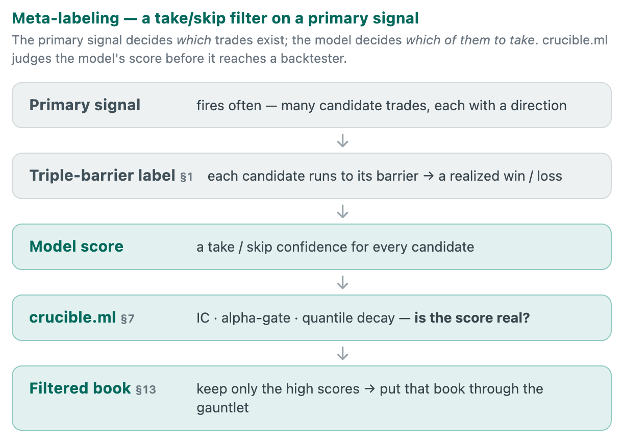Meta-labeling splits the decision: the primary signal decides which trades exist, the model decides which to take. crucible.ml judges the model's score before it ever reaches a backtester, the pipeline §13 runs end to end.

Sources. AFML Ch. 3 "Labeling," §3.4 "The Triple-Barrier Method" (with §3.5 "Learning Side and Size" and §3.6 "Meta-Labeling"), the labeling and take/skip framing.

Is the ML score real? crucible.ml

Code: ml/ic.py, ml/decay.py, ml/redundancy.py, ml/pit.py

Once a model emits a score, the same honesty question §4 asks of a trade log applies to the score: does a higher score actually rank better outcomes, or is it noise, leakage, or a feature wearing a new name? crucible.ml answers it capital-free (numpy/pandas only), on the model's predictions rather than an equity curve.

• Information Coefficient (information_coefficient), the Spearman rank correlation between a score and its realized label. Rank-based, so it's invariant to the label encoding (+1/−1 or 0/1) and to any monotonic transform of the score: it measures only whether higher scores line up with better outcomes. alpha_gate(ic, min_ic=…) raises below the bar, a PASS/FAIL you wire into a training loop to kill an edge-less or leaking model before it reaches a backtester. Computed out-of-fold (fold_ic), and, echoing §5, its sign-stability across folds matters more than its magnitude: a weak-but-consistently-positive IC is a better sign than a strong one that flips.

• Quantile decay (quantile_decay), bucket the score into equal-count quantiles and read the realized win rate per bucket. A genuine, well-ordered edge makes win rate climb monotonically Q1→Q5 (.monotonic, .spread). A flat or ragged profile is the tell of a score that ranks nothing. decay_tearsheet renders it as self-contained HTML.

• Feature redundancy (redundancy_droplist), clusters features by |Spearman| / Cramér's V and keeps the highest-|IC| member of each cluster. This is the feature-space analogue of §10's N_eff: three features that are one feature in disguise are one bet, not three, and counting them as independent inflates any significance claim downstream.

• Point-in-time slices (asof_window / window_before), a leakage-safe window so a live feature is built identically to its training twin: the feature-space cousin of §8's purge/embargo. §8 stops the label from peeking ahead. This stops the features from doing so.

Sources. The Information Coefficient and the link between per-bet skill and portfolio performance: Grinold & Kahn, Active Portfolio Management (the IC and the Fundamental Law of Active Management), outside the six-book set, but the canonical IC reference. Out-of-fold feature importance, judging features on unseen data: AFML Ch. 8 "Feature Importance." No-look- ahead feature construction: AFML Ch. 7 §7.4, the purge/embargo principle applied to features. Quantile-decay monotonicity is the standard factor-research check (the alphalens lineage).

---

8. Confirming out-of-sample: holdout, purge & embargo

The test period is worth exactly one look. This is how not to waste it.

Code: validation/holdout.py. holdout, split_train_test

For a fixed strategy, the honest test is temporal: measure the edge early, freeze it, confirm on a late period the analysis never touched. Two leakage controls make the split real (holdout.py:36-48):

• Purge: a training trade must have both entered and exited before the split, a trade whose forward window straddles the boundary can't leak future information into the fitted side.
• Embargo: drop the first embargo_weeks of the test period, killing residual autocorrelation across the seam.

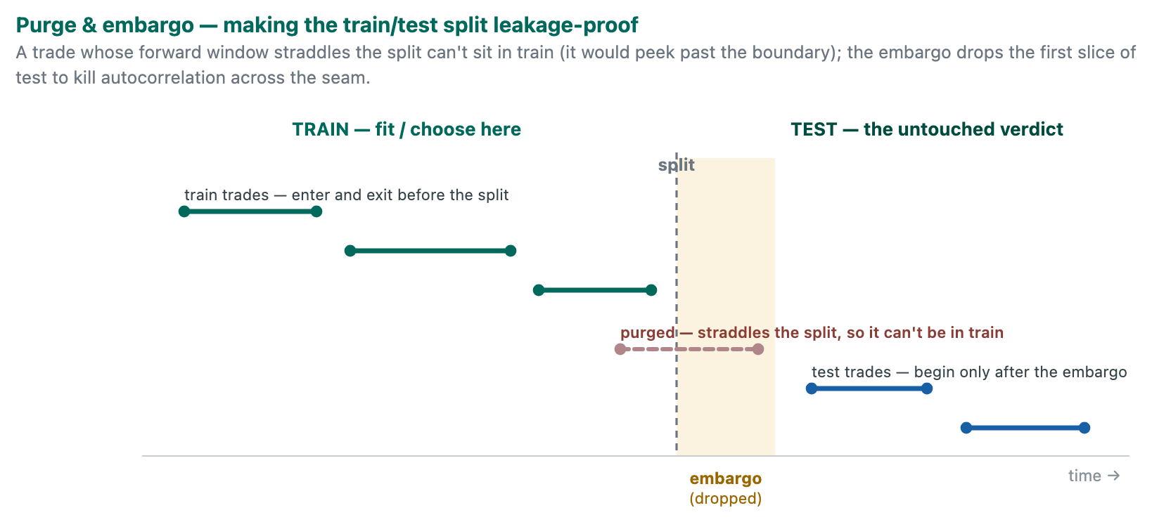Purge removes any trade whose forward window crosses the split (it would carry future information into the fitted side). Embargo drops the first slice of test so autocorrelation can't leak across the seam. What remains on the right has genuinely never been seen.

The HoldoutResult runs a full reality_check on each side and declares the untouched TEST period the verdict (holdout.py:56, :69). Train is expected to look good. That's where an edge would have been chosen. Only test counts.

What's being fitted when nothing is being optimized

That last sentence hides the part that matters. If you come from a tool where "in-sample" means an optimizer swept a grid, then applying a holdout to a fixed strategy looks like ceremony. In-sample what? Nothing was fit. No solver ran. The parameters were never touched.

But the holdout was never protecting you from the optimizer. It protects you from you. Every rule change you made after looking at a result is a fit: you saw the equity curve, you responded, and the response was chosen because of what you saw. That is the same act an optimizer performs, executed by hand and at a much lower sample rate. The optimizer's one real virtue is that it counts, the grid is self-documenting, and the tool hands you the trial number. A human search leaves no record at all, which is exactly what makes it the more dangerous of the two.

So the discipline is unchanged even with no solver in the loop: the train period is the only place you are allowed to look. Every glance at test is a fit to test, whether or not any software registered it, and it spends the one thing the test period has, never having been seen. Once spent, a "holdout" is just more train.

Note the contrast with §9, where a real optimizer does run: walk_forward picks the best lookback in-sample per fold, machine-fit and machine-counted. Both are IS → OOS and the logic is identical. The difference is only who did the fitting and who has to do the counting, and here, that's you.

Sources. - AFML Ch. 7 "Cross-Validation in Finance," §7.4 "A Solution: Purged K-Fold CV", the origin of purge + embargo for overlapping financial labels. - Pardo (2008), the "Walk-Forward Analysis" chapter, the in-sample/out-of-sample discipline this generalizes. - Carver, Systematic Trading, Ch. 3 "Fitting", why in-sample results prove nothing and the case for simple, robust, hard-to-overfit parameters.

---

9. Confirming it keeps working: walk-forward analysis & efficiency

The one test you already run, and the two instincts that make you misread it.

Code: validation/walk_forward.py. walk_forward, _wfe

One holdout is a single split. walk-forward rolls it through history: optimize params on an in-sample window, apply the winner to the next untouched out-of-sample window, step forward, repeat, then stitch all OOS slices into one trade log. If the stitched OOS edge survives reality_check, the strategy generalized through time. If it dies, the in-sample result was curve-fit (walk_forward.py module docstring).

Each fold carries the same purge/embargo hygiene (purge_days, embargo_days, walk_forward.py:136-138) and reports Walk-Forward Efficiency (WFE), Pardo's named ratio of annualized OOS return / annualized IS return (_wfe, :47). WFE ≈ 50–80% is healthy. Below ~30% is fragile, above 100% is "too good to be true" (usually a bug or luck).

Two instincts carried over from the equity-curve world will quietly invert the result.

The first is that higher WFE is better. It isn't. The metric has a ceiling, not just a floor. WFE is out-of-sample over in-sample, so a WFE above 1.00 says your strategy did better on data it had never seen than on the data it was fitted to. That is not a triumph. It's a statement that something is wrong, and wfe_reject_high = 1.00 (thresholds.py:29) rejects it outright. Usually it's a bug, a leak, or a couple of freak folds, but whatever it is, it isn't skill, because fitting is supposed to help on the data you fit to. §12 fails on exactly this.

The second is that the aggregate is the answer. It's a mean, and means get carried. A healthy aggregate WFE can be a strategy that was mediocre in most of its folds and extraordinary in two, and those two are the least likely to repeat, because outliers are the thing that doesn't. Read the fold column, not the summary row. (§12 is this exact shape: an aggregate of 1.34 with individual folds at 3.5 and 3.7.)

crucible's DURABLE gate hardens this against a specific trap (fold_dispersion in validation/diagnostics.py): a healthy average WFE can hide individually chaotic folds, so it adds a fold-dispersion check, what fraction of folds are individually tradable (SQN > 0) and the coefficient of variation of fold SQN. High dispersion is itself a rejection, independent of the average.

Sources. - Pardo (2008), the walk-forward method and the Walk-Forward Efficiency metric are his. The WFA chapter is the primary source. walk_forward.py is a capital-free reimplementation of it. - AFML Ch. 12 "Backtesting through Cross-Validation," §12.2 "The Walk-Forward Method" and §12.4 "The Combinatorial Purged Cross-Validation Method", the modern critique and generalization of single-path walk-forward. - SSML Introduction, "Walkforward Testing" and "Overlap Considerations."

---

10. Correcting for correlation: effective sample size & portfolio survivability

You counted every market as a fresh confirmation. Most of them were the same bet.

A book of 665 trades across 20 markets is not 665 independent bets: eight currency futures are roughly one dollar bet. Two tools account for this: one capital-free and native to crucible, one capital-aware and out of crucible's scope. Both bear directly on whether a significance claim is honest.

Effective N, breadth.py: effective_n(returns) returns a Breadth whose n_eff = (Σλ)² / Σλ² is the participation ratio of the eigenvalues of the return-correlation matrix (participation_ratio). N perfectly independent markets give N_eff = N. Perfectly correlated give N_eff = 1. It is "the honest denominator for significance", a permutation p-value computed as if trades were independent is optimistic when they cluster into a few factors, which the returned PCA loadings then name (dollar / rates / grains / …). Capital-free: correlation structure only, no equity curve.

>>> from crucible.breadth import effective_n
>>> effective_n(returns).n_eff     # 20-market book, ~3 correlated blocs + a lone metal
3.8                                # ...so it's really ~4 independent bets

Portfolio Monte Carlo is the capital-aware sibling, deliberately out of crucible's scope, because it needs a capital model crucible doesn't have. The idea: a circular block bootstrap of the monthly portfolio-return series (contiguous blocks preserve the clustering and autocorrelation a naive per-trade shuffle destroys) yields a distribution of max drawdown, terminal equity, and risk-of-ruin per risk fraction. crucible.breadth measures the independence structure. The drawdown consequence of it is the SURVIVE handoff (§11). Hand the TradeLog to a capital-aware tool.

Sources. - Concurrency / overlap and effective sample size: AFML Ch. 4 "Sample Weights," §4.3 "Number of Concurrent Labels" and §4.4 "Average Uniqueness of a Label". Correlation- based structure in Ch. 16 "Machine Learning Asset Allocation" (HRP. §16.A.1 "Correlation-Based Metric"). - Number of independent bets and the diversification multiplier: Carver, Systematic Trading, Ch. 11 "Portfolios" and Appendix D "Framework Details → Calculation of diversification multiplier". Extended in Carver, Advanced Futures Trading Strategies (instrument diversification and its multiplier across a large universe). - Monte Carlo drawdown / risk-of-ruin on reshuffled trade sequences: Pardo (2008), Monte Carlo and money-management material. Risk of ruin and strategy failure: AFML Ch. 15 "Understanding Strategy Risk," §15.4 "The Probability of Strategy Failure." - Position sizing, the SURVIVE layer crucible hands off, is the subject of Van Tharp, Definitive Guide to Position Sizing (2008) (risk / volatility / percent-of-equity models), Tom Basso, Successful Traders Size Their Positions: Why and How? (2019) (risk %, volatility %, capital/margin, portfolio-heat), and Carver, Systematic Trading, Ch. 10 "Position Sizing" (turning the volatility target of §1's Ch. 9 into an actual position).

---

11. The whole pipeline, as one gate: crucible.validation.run_gauntlet

Every technique above, wired into one audited pass/fail that nobody gets to argue with.

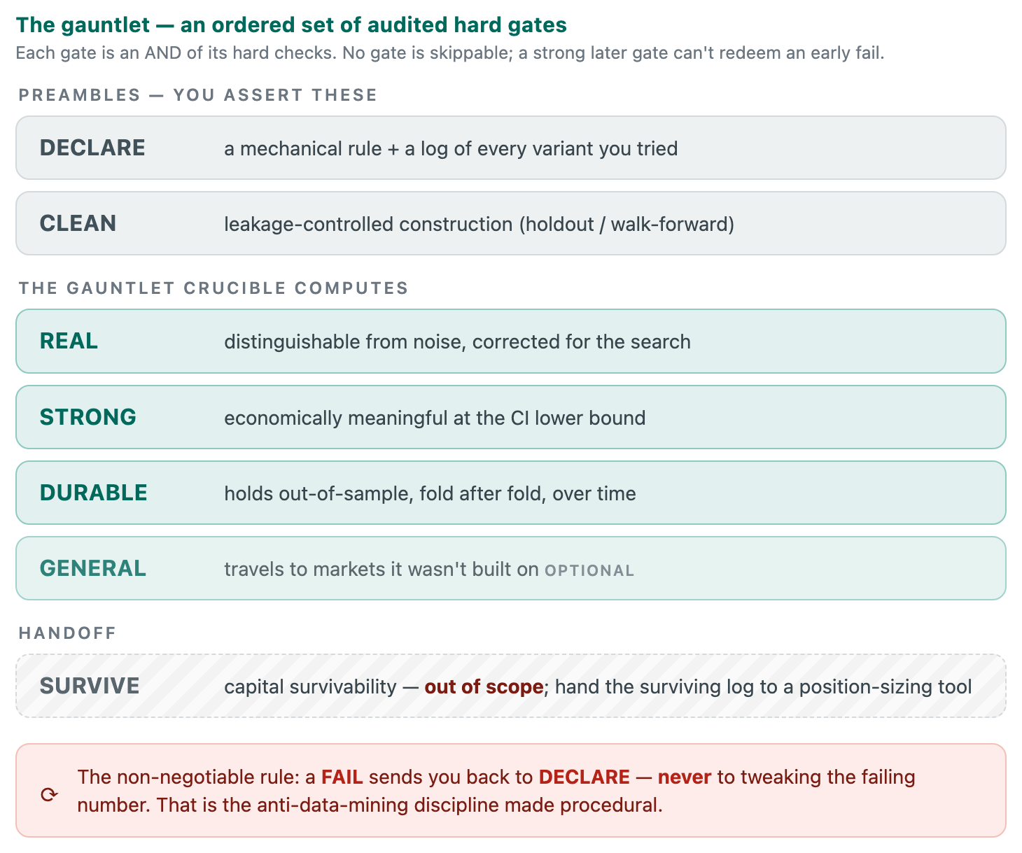
Every primitive above answers one question. The gauntlet runs them as an ordered set of audited hard gates and returns a single, capital-free pass/fail, crucible's own naming, no stage numbers borrowed from anywhere:

from crucible.validation import run_gauntlet

gauntlet = run_gauntlet(
    wf.stitched,        # the honest log, stitched out-of-sample
    prices=px,          # enables REAL's random-entry null
    wf=wf,              # adds the DURABLE gate
    n_variants=4,       # size of your search -> REAL's Šidák correction
)
print(gauntlet.audit_report())
print(gauntlet.passed)  # True only if every gate that ran passed

Read the table by the claim: find the sentence you want to be able to say out loud, and the gate is what earns you the right to say it.

Gate	the claim it earns	Built from
DECLARE (preamble)	"the rule is mechanical, and I've admitted what I tried"	EBTA Ch. 1 (§0). The variant count feeds §5
CLEAN (preamble)	"I'm not reading the future"	purge/embargo (§8). The look-ahead-free simulator (§1)
REAL	"it isn't luck, it isn't my search, and it isn't just a market that went up"	permutation + Šidák / White's Reality Check (§5). Random-entry null (§6)
STRONG	"it's big enough to matter, at the CI lower bound, not my point estimate"	edge metrics (§2), bootstrap CIs (§3)
DURABLE	"it keeps working"	walk-forward + WFE + fold dispersion (§9)
GENERAL	"it isn't only this one market"	cross-market Reality Check (§5e). Breadth / N_eff (§10)
SURVIVE (handoff)	"I can actually trade it"	out of scope (position sizing, drawdown, ruin)

Each gate is an audited AND of its hard checks, a failing hard check can't be waived, and a strong later gate can't redeem an early failure. The non-negotiable rule: a FAIL sends you back to DECLARE, never to tweaking the failing number. That is the anti-data-mining discipline made procedural, and that loop is also the counter §5b asked you for: every trip back around is n_variants += 1. Going back to DECLARE is allowed and expected. Going back having forgotten the last attempt is what turns an honest p-value into a lie. Full write-up in docs/edge_gate.md.

The gauntlet as a report: gauntlet_report() / tearsheet()

crucible.report renders the same verdict as a self-contained, theme-aware HTML page (the [report] extra adds plotly): a verdict banner and pillar chips, the metric row, the edge charts, and one expandable block per gate. It visualizes the edge, never an account, no equity curve, no capital.

from crucible.report import gauntlet_report
gauntlet_report(gauntlet, wf.stitched, path="gauntlet.html")   # one self-contained file

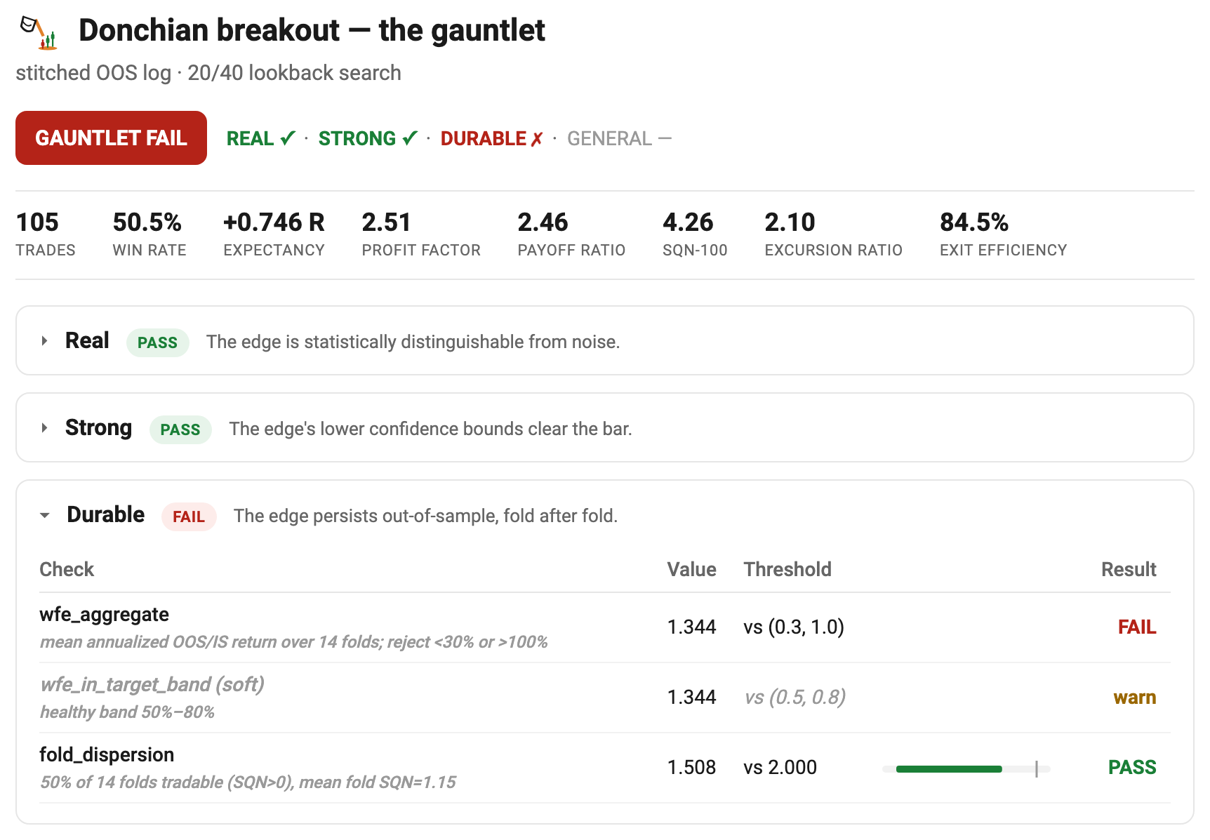The verdict banner and pillar chips, the metric row, then one block per gate. Each block states its plain-English claim and its PASS/FAIL, and the failing gate expands to the exact checks and thresholds. tearsheet() renders a single book the same way.

The verdict reads in three states, not two

REAL / STRONG / DURABLE answer "is the edge real?", the core question. GENERAL answers a separate one, "does it generalize beyond the markets it was built on?", so the report frames the banner in three states rather than a flat pass/fail:

• GAUNTLET PASS (green): every gate that ran passed.
• EDGE VALIDATED · scope-limited (amber): the core (REAL/STRONG/DURABLE) holds and the only miss is GENERAL. The edge is real and deployable on the markets it was built on. Only its cross-market reach is unproven. That's a documented scope boundary, not a rejected edge. Trade the set it's proven on rather than extrapolating to new markets on faith.
• GAUNTLET FAIL (red): a core gate missed, so the edge itself is in question.

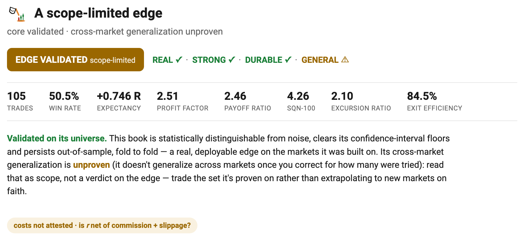Same report, amber instead of red: a GENERAL-only miss is a bounded-scope caveat, not a failed edge. This is a presentation distinction, gauntlet.passed stays strict (True only if every gate that ran, GENERAL included, passed), so a scope-limited book still returns passed == False. The gate math and thresholds are unchanged. Only the framing is.

---

12. Worked example: a Donchian breakout, read end to end

A profit factor of 1.90, taken apart on the page. It does not survive.

Everything above, run as one script on a Donchian channel breakout: go long when price closes above the prior 20-bar high. Exit on a 2.5R target, a 1R stop, or a 30-bar cap. The full runnable version is in examples/donchian_gauntlet.py; it uses reproducible synthetic prices, so you can run it with no network and get these exact numbers.

The whole pipeline you're about to run, at a glance — from the trade log through the gates to one of three verdicts:

flowchart TD
    IN["Trading strategy R-multiples"]
    DECLARE["Declare (you bring this)<br/>Mechanical rule + variant count (N)"]
    CLEAN["Clean (you bring this)<br/>Leakage-free: purge and embargo"]
    REAL["1 · Real<br/>Search-corrected significance<br/>permutation + Šidák vs random-entry null"]
    STRONG["2 · Strong<br/>Expectancy, profit factor, SQN<br/>at the 95% CI lower bound"]
    DURABLE["3 · Durable<br/>Walk-forward efficiency + fold dispersion"]
    GENERAL["4 · General (optional)<br/>Cross-market reality check"]
    PASS["Gauntlet pass<br/>every gate that ran passed,<br/>including the optional general gate"]
    AMBER["Edge validated — scope-limited<br/>core gates pass, general fails<br/>real, but only for the proven markets"]
    FAIL["Gauntlet fail<br/>any core gate fails — stop here<br/>likely an artifact of noise or overfitting"]

    IN --> DECLARE --> CLEAN --> REAL --> STRONG --> DURABLE --> GENERAL
    GENERAL -->|all gates pass| PASS
    GENERAL -->|general fails| AMBER
    REAL -.->|any core gate fails| FAIL
    STRONG -.-> FAIL
    DURABLE -.-> FAIL

    classDef pre stroke:#888780,stroke-width:1.5px;
    classDef core stroke:#1D9E75,stroke-width:2px;
    classDef opt stroke:#7F77DD,stroke-width:2px;
    classDef pass stroke:#639922,stroke-width:2px;
    classDef amber stroke:#BA7517,stroke-width:2px;
    classDef fail stroke:#E24B4A,stroke-width:2px;

    class IN,DECLARE,CLEAN pre;
    class REAL,STRONG,DURABLE core;
    class GENERAL opt;
    class PASS pass;
    class AMBER amber;
    class FAIL fail;

from crucible.edge import barrier_trades, edge_report, reality_check
from crucible.validation import walk_forward, run_gauntlet

def donchian(df, lookback=20):
    return df["Close"] > df["High"].rolling(lookback).max().shift(1)

entries = donchian(px, lookback=20)                                  # your signal
trades  = barrier_trades(px, entries, side="long", tp=2.5, sl=1.0, timeout=30)

Step 1: describe the edge (§2)

edge_report(trades)
   Trades        : 162          Payoff ratio  : 2.50
   Win rate      : 43.2 %       SQN-100       : 2.95
   Expectancy    : +0.512 R     Excursion     : 1.77   [PASS]
   Profit factor : 1.90         Time asymmetry: 2.19   [PASS]

How to read it. A textbook trend-following shape: a low win rate (43%) paired with a payoff of 2.5 (winners run about 2.5× the size of losers) nets a positive expectancy and PF 1.90. Excursion and time-asymmetry both above 1 say the signal has directional edge before the exit rule even acts. But these are point estimates on 162 trades: they describe, they don't yet defend. SQN 2.95 hints the sample can support a claim. Keep going.

Step 2: is it real, or small-sample luck? (§3–§4)

reality_check(trades)
   VERDICT (expectancy): +0.512 R   95% CI [+0.253, +0.772]
                         p(edge>0) = 1.000   ->  HELD

How to read it. The bootstrap CI lower bound (+0.253) clears zero. Across 10,000 resamples the edge stays positive. Verdict HELD: on the whole history this is not small-sample noise. A backtester would stop right here, with a rising equity curve. crucible doesn't. HELD on the pooled log is necessary, not sufficient.

Step 3: does it survive out of sample, over time? (§9)

walk_forward(px, donchian, {"lookback": [20, 40]}, is_days=3yr, oos_days=1yr)
   OOS year   IS E     OOS E    WFE          OOS year   IS E     OOS E    WFE
   2011      +0.925   +2.150   3.52          2016      +1.000   −1.000  −0.14
   2012      +1.258   +1.227   1.40          …
   2013      +1.220   +1.000   0.71          2022      +0.690   +0.969   3.66
   2014      +1.214   −1.000  −0.31          2023      +0.716   +0.925   3.77
   2015      +1.087   −0.125  −0.06          folds=14  mean WFE=1.34  stitched=105

How to read it. Optimize the lookback in-sample, apply the winner to the next unseen year, step forward, stitch the out-of-sample slices into one log. The in-sample expectancy is steadily positive, but the OOS column lurches: +2.15, +1.23, +1.00, then −1.00, −0.13, −1.00 … a few great years and a run of losing ones, and only half the years profitable. The mean WFE of 1.34 looks respectable until you notice it's above 1.00, the out-of-sample outran the in-sample, which §9 flagged as too-good-to-be-true. A few outlier years (fold WFEs of 3.5, 3.7, 5.3) inflated the average. Step 4 makes the call.

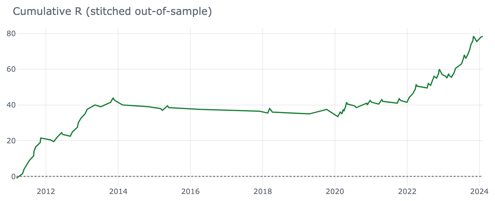The stitched out-of-sample slices as one cumulative-R curve, an early climb, a long flat/choppy middle (the losing years), then a late rip a few outlier years drive. Convincing as a curve. The gauntlet still rejects it.

Step 4: the verdict (§11)

run_gauntlet(wf.stitched, prices=px, wf=wf, n_variants=2)
   REAL     ✓   corrected p = 0.0008   ·   beats 100% of random-entry timing
   STRONG   ✓   expectancy CI-low +0.40 · PF CI-low 1.67 · SQN CI-low 2.32
   DURABLE  ✗   wfe_aggregate 1.34 above the [0.30, 1.00] ceiling  ·  fold_dispersion CV 1.51 → PASS
   ─────────────────────────────────────────────────────────────────────
   GAUNTLET: FAIL   (2 of 3 gates passed, failing: DURABLE)

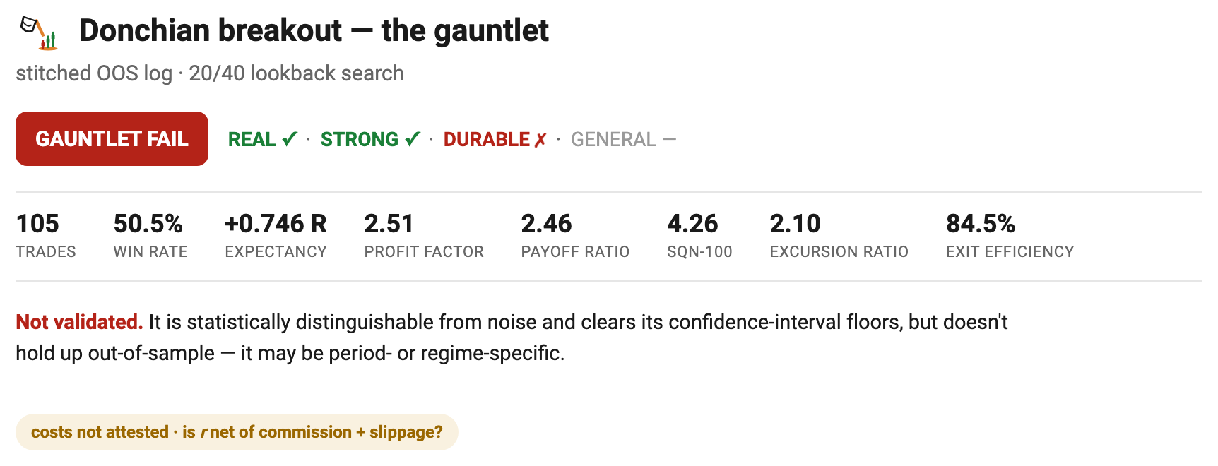The same verdict as gauntlet_report() renders it (§11): pillar chips, the metric row, and a plain-English read, real and strong, but not durable, so not validated. This run fails on DURABLE, a core gate, so it's a genuine red FAIL. Had REAL/STRONG/DURABLE held and only GENERAL missed, the same report would read amber, EDGE VALIDATED · scope-limited (§11).

Reading it gate by gate:

• REAL ✓, the sign-permutation p is 0.0008 (well under 0.05, Šidák-adjusted for the 2 lookbacks searched), and the expectancy beats 100% of random-entry books on the same prices. Not noise, and not just riding the drift: real timing edge.
• STRONG ✓, every hard metric clears its bar at the pessimistic CI lower bound, not the point estimate: expectancy-low +0.40 (> 0), PF-low 1.67 (> 1.25), SQN-low 2.32 (> 1.6). Economically real even under sampling noise.
• DURABLE ✗, and here it dies. The aggregate WFE is 1.34, above the 1.00 "too-good-to-be-true" ceiling: the out-of-sample outran the in-sample, inflated by a few outlier years (fold WFEs of 3.5–5.3), the opposite of the graceful 50–80% degradation a robust edge shows. Fold dispersion itself passes, but barely, only half the folds are individually tradable (CV 1.51 vs. a bar of 2.0).

The lesson. Pooled, and even out-of-sample in aggregate, this breakout is real and strong: reality_check said HELD, and two of three gates are green. A backtester's equity curve would have sold it to you. But DURABLE, the gate crucible won't let you skip, exposes it. The edge doesn't hold up through time. Overall FAIL: back to DECLARE, don't size it up. That is the whole reason to run the gauntlet instead of trusting a curve.

A PASS reads the same way with three green gates and GAUNTLET: PASS, an edge that's real, strong, and durable, leaving only SURVIVE (capital), which you take to a position-sizing tool (§10's sources). Most naive signals look like this Donchian: convincing on the surface, caught by DURABLE or REAL.

---

13. Worked example: an ML take/skip filter, read end to end

The score is real, which is not the same as the book being strong. Watch a marginal edge cross the line.

The ML track (§7) run as one script on a meta-labeling take/skip filter: a primary signal has already produced a book of candidate trades, and a model scores each one, take it or skip it. The full runnable version is in examples/ml_meta_label.py; it uses a reproducible synthetic book (no network), so you can run it and get these exact numbers.

from crucible.ml import information_coefficient, alpha_gate, quantile_decay, fold_ic
from crucible.validation import run_gauntlet
from crucible.edge import TradeLog

book  = synthetic_meta_book()          # 1,600 candidate trades: score, label, r
preds = book[["score", "label"]]       # the model's score and the realized win/loss

Each candidate carries a hidden edge quality. The model's score reads that quality imperfectly, a real but noisy signal, never the label itself. The first two questions are §7's, the third is §11's.

Step 1: is the score real? (§7)

information_coefficient(preds)   IC = +0.218          alpha_gate(min_ic=0.03): PASS
fold_ic(book, ["score"])         out-of-fold IC = +0.214 ± 0.061   (positive in all 5 folds, IR +3.53)

How to read it. The Information Coefficient is the rank correlation between score and outcome: +0.218 says higher scores really do rank better trades, and alpha_gate passes it. But the number that carries more weight is the out-of-fold one (measured on trades the score didn't see) and its sign-stability: +0.214, positive in every one of the five folds. Per §7, a consistently-positive IC beats a bigger one that flips sign fold to fold. This one never flips. That out-of-fold split is also what keeps it honest, a score fit and judged on the same trades would be the §8 leakage mistake.

Step 2: does the score rank outcomes? (§7)

quantile_decay(preds, q=5)
   score quantile    Q1      Q2      Q3      Q4      Q5
   win rate        26.6%   34.1%   37.2%   45.0%   57.8%     monotonic ✓   spread +31 pts

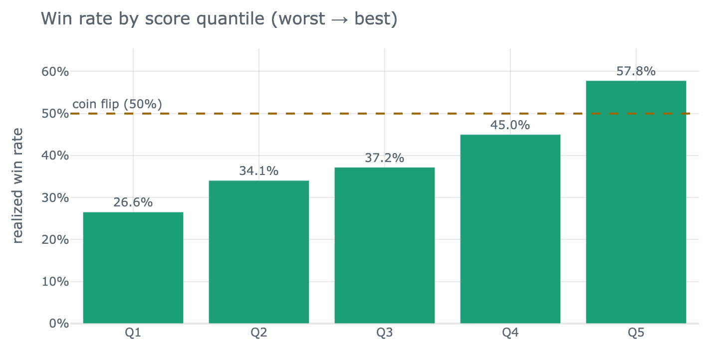The decay picture §7 describes: bucket the score into fifths, read the realized win rate per bucket. A real, well-ordered score makes win rate climb monotonically, here 26.6% → 57.8%, a +31-point spread, crossing the 50% coin-flip line only in the top quantile.

How to read it. IC gives one number. The decay shows its shape. Win rate climbs every bucket, Q1 to Q5, the mark of a score that orders trades, not one lucky bucket carrying the average. And notice where 50% is crossed: only the top quantile wins more often than a coin. That is the meta-labeling thesis in a picture, the edge lives in the high scores.

Step 3: does the filter pay? (§11)

Take the top 40% by score, and put both books, the whole primary book and the filtered one, through the gauntlet. (No price series or multiple markets here, so this is the trade-log gauntlet: REAL + STRONG. DURABLE and GENERAL would need §9's walk-forward and §10's breadth.)

                     trades    win        E        PF     gauntlet
   unfiltered         1600    40.1%    +0.197R    1.33    REAL ✓ · STRONG ✗   → FAIL
   filtered (top 40%)  640    51.4%    +0.538R    2.11    REAL ✓ · STRONG ✓   → PASS

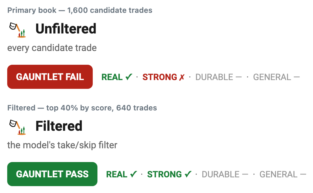Same book, split on the score: the primary book (top) is real but not strong. The top-40% book (bottom) clears both gates.

How to read it, and this is the whole point. The primary book is real but not strong, and why it fails STRONG is the lesson: its profit factor is 1.33, comfortably over the 1.25 bar. But STRONG gates the CI lower bound, not the point estimate (§3, §11), and the PF lower bound is 1.20, under the bar. The point estimate looked fine. The honest, pessimistic read did not. This is exactly the trap §0's table named, "the same 1.37 with a CI around it", now landing on an ML book.

The filter fixes it by construction: keep only the top-score trades and win rate climbs 40% → 51%, expectancy nearly triples (+0.197R → +0.538R), and PF rises to 2.11, whose lower bound now clears 1.25 with room. REAL ✓ · STRONG ✓ · PASS. Meta-labeling turned a marginal edge into a strong one, not by finding a new signal, but by declining the bottom of the one it already had.

The lesson. A score can be genuinely real (Step 1) and cleanly ordered (Step 2) and still leave you a book that misses STRONG (Step 3, unfiltered): "the score is real" and "the book is strong" are different claims, and only the gauntlet separates them. The filter earns its keep because the filtered book passes at the CI lower bound, but read the trade count, 1,600 → 640. Filtering is not free. It spends sample, and take too little and STRONG fails the other way, on a CI too wide to clear the bar (§3). The take/skip model is itself a fitted thing, so it owes the same discipline as any book: out-of-fold scoring (Step 1), a holdout on the selection (§8), and its search counted in n_variants (§5). Real, strong, and honestly filtered, then it goes on to DURABLE and the rest of the ladder, same as any other edge.

---

Bibliography

Listed in rough order of contribution to the significance machinery. Items 1–6 are the significance canon, "the six-book set" referenced above. 7–8 cover the position-sizing (SURVIVE) layer crucible hands off. Where a book is organized by topic rather than fixed pagination (SSML) or where I cite a chapter rather than a verified page, that is stated explicitly.

1. Aronson, David R., Evidence-Based Technical Analysis (Wiley, 2006/2007). The statistical backbone. Ch. 4 "Statistical Analysis" (p. 165). Ch. 5 "Hypothesis Tests and Confidence Intervals" (p. 217) → bootstrap CIs, hypothesis testing. Ch. 6 "Data-Mining Bias: The Fool's Gold of Objective TA" (p. 255) → the permutation test, White's Reality Check, multiple comparisons. Ch. 8 "Case Study of Rule Data Mining for the S&P 500" (p. 389) → the method applied to 6,402 rules. Appendix "Proof That Detrending Is Equivalent to Benchmarking Based on Position Bias" (p. 475) → the detrended benchmark. Acknowledgments (p. ix) credit Timothy Masters with the Monte Carlo permutation method.

2. Aronson, David R. & Masters, Timothy, Statistically Sound Machine Learning for Algorithmic Trading of Financial Instruments (2013). Applied companion to EBTA, organized by topic around the TSSB tool. Introduction → "Walkforward Testing," "Cross Validation," "Overlap Considerations," "Performance Criteria," "Model Performance Versus Financial Performance," "Financial Relevance and Generalizability". Plus the permutation- test / selection-bias sections. Source for the sign-permutation implementation and the model-vs-financial-performance distinction.

3. López de Prado, Marcos, Advances in Financial Machine Learning (Wiley, 2018). The leakage-control and ML-labeling backbone. Ch. 3 "Labeling" §3.4 "The Triple-Barrier Method," §3.6–3.7 "Meta-Labeling". Ch. 4 "Sample Weights" §4.3–4.4 (concurrency, uniqueness → effective sample). Ch. 7 "Cross-Validation in Finance" §7.4 "Purged K-Fold CV" (purge & embargo). Ch. 11 "The Dangers of Backtesting". Ch. 12 "Backtesting through Cross-Validation" §12.2 (walk-forward), §12.4 (CPCV). Ch. 14 "Backtest Statistics". Ch. 15 "Understanding Strategy Risk" §15.4 "The Probability of Strategy Failure". Ch. 16 "ML Asset Allocation" (correlation structure).

4. Pardo, Robert, The Evaluation and Optimization of Trading Strategies, 2nd ed. (Wiley, 2008). The temporal-robustness backbone. The "Evaluation of Trading Strategies" chapter → the classic performance metrics (edge_report). The "Walk-Forward Analysis" chapter → walk-forward method and the Walk-Forward Efficiency (WFE) metric. The optimization/robustness and Monte-Carlo money-management material. (Cited by chapter; the scanned copy's page numbers were not individually verified here.)

5. Carver, Robert, Systematic Trading (Harriman House, 2015). Overfitting discipline and portfolio structure. Ch. 3 "Fitting" → in-sample/out-of-sample, robust simple parameters. Ch. 9 "Volatility Targeting" → the volatility risk unit behind R-normalized returns (§1), Ch. 10 "Position Sizing" → the sizing handoff (SURVIVE, §11). Ch. 11 "Portfolios" and Appendix C "Portfolio Optimisation" (bootstrapping, rule-of-thumb correlations) and Appendix D "→ Calculation of diversification multiplier" → the number-of-independent-bets idea behind N_eff.

6. Carver, Robert, Advanced Futures Trading Strategies (Harriman House, 2021). Referenced to a lesser extent. The Sharpe-ratio / return-evaluation chapters (a performance statistic is itself an estimate with error) and the instrument-diversification / diversification-multiplier material across a large futures universe, the practical counterpart to crucible.breadth and the portfolio Monte Carlo crucible hands off (§10). (Cited at concept/chapter level.)

7. Van Tharp, Van K., Definitive Guide to Position Sizing (IITM, 2008) and Trade Your Way to Financial Freedom, 2nd ed. (McGraw-Hill, 2007). The R/SQN origin and the position-sizing layer. Definitive Guide Ch. 2 "Risk (R) and R-Multiples" (p. 11) → §1's R-multiple. Ch. 3 "Evaluating the Quality of Your Trading System" (p. 23), with "One Problem with SQN and How to Overcome It" (p. 32) and "Statistical Assumptions" (p. 33) → the SQN and its small-sample caveat (§2). Its position-sizing parts are the SURVIVE layer crucible hands off. ("R," "SQN," "Position Sizing" are Tharp / IITM service marks.)

8. Basso, Tom, Successful Traders Size Their Positions: Why and How? (enjoytheride.world, 2019). Position sizing only, the SURVIVE layer. Risk %, volatility %, capital/margin, and portfolio-heat sizing, the capital methodology crucible stops short of and hands off (§10).

Supporting references (papers, not in the six-book set): White, Halbert (2000), "A Reality Check for Data Snooping," Econometrica 68(5): 1097–1126 → the Reality Check whites_reality_check reimplements.  ·  Bailey & López de Prado (2014), "The Deflated Sharpe Ratio," J. Portfolio Management, and Bailey, Borwein, López de Prado & Zhu (2017), "The Probability of Backtest Overfitting," J. Computational Finance → §5's deflated_sharpe / pbo_cscv.  ·  Grinold & Kahn, Active Portfolio Management → the Information Coefficient (§7).

---

Code map (where each technique lives)

Technique	File
Trade-log schema, R-multiples	crucible/src/crucible/edge/trade_log.py
Look-ahead-free barrier simulator	crucible/src/crucible/edge/simulator.py
Edge metrics (expectancy, PF, SQN, excursion…)	crucible/src/crucible/edge/metrics.py
Bootstrap CI + metric-set CIs, p-value, reality_check verdict	crucible/src/crucible/edge/stats.py
Block/stationary-bootstrap significance (serial dependence)	crucible/src/crucible/edge/stats.py
Random-entry null + detrended timing null	crucible/src/crucible/edge/stats.py
Sign-permutation, Šidák, White's Reality Check + Hansen's SPA	crucible/src/crucible/validation/permutation.py
PBO (CSCV) + deflated Sharpe	crucible/src/crucible/validation/pbo.py
ML signal quality: IC, decay, redundancy, PIT	crucible/src/crucible/ml/
Purged/embargoed holdout	crucible/src/crucible/validation/holdout.py
Walk-forward + WFE	crucible/src/crucible/validation/walk_forward.py
Fold dispersion / WFE diagnostics	crucible/src/crucible/validation/diagnostics.py
Audited gate + Gauntlet	crucible/src/crucible/validation/gate.py
The gauntlet (REAL/STRONG/DURABLE/GENERAL) + Thresholds	crucible/src/crucible/validation/gauntlet.py
Effective N / factor PCA	crucible/src/crucible/breadth.py
Worked example (Donchian breakout, §12)	crucible/examples/donchian_gauntlet.py
Worked example (ML take/skip filter, §13)	crucible/examples/ml_meta_label.py

---

Appendix: the underlying statistics, on Wikipedia

Convenience look-ups for the techniques above, secondary to the primary sources in the bibliography, not a replacement for them.

Concept	In	Wikipedia
Bootstrapping (resampling)	§3	Bootstrapping (statistics)
Block / stationary bootstrap (dependent data)	§3	Bootstrapping (statistics)
Confidence interval	§3	Confidence interval
Permutation test	§5	Permutation test
Data-mining bias	§5	Data dredging
White's Reality Check / SPA test (no dedicated pages)	§5	Data dredging · Peter Reinhard Hansen
Multiple comparisons	§5	Multiple comparisons problem
Šidák correction	§5	Šidák correction
Backtest overfitting / deflated Sharpe	§5	Deflated Sharpe ratio
Sharpe ratio	§5	Sharpe ratio
Cross-validation	§5, §9	Cross-validation (statistics)
Walk-forward optimization	§9	Walk forward optimization
Information coefficient	§7	Information coefficient
Spearman rank correlation	§7	Spearman's rank correlation coefficient
Skewness & kurtosis	§5	Skewness · Kurtosis
Principal component analysis	§10	Principal component analysis
Monte Carlo method	§10	Monte Carlo method